Goertzel algorithm
The Goertzel algorithm is a digital signal processing (DSP) technique for identifying frequency components of a signal, published by Gerald Goertzel in 1958[1]. While the general Fast Fourier transform (FFT) algorithm computes evenly across the bandwidth of the incoming signal, the Goertzel algorithm looks at specific, predetermined frequencies.
A practical application of this algorithm is recognition of the DTMF tones produced by the buttons pushed on a telephone keypad[2][3][4].
It can also be used "in reverse" as a sinusoid synthesis function, which requires only 1 multiplication and 1 subtraction per generated sample.[5][6]
Contents |
Explanation of algorithm
The Goertzel algorithm computes a sequence,  , given an input sequence,
  :
:

where 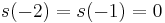 and
and  is some frequency of interest, in cycles per sample, which should be less than 1/2. This effectively implements a second-order IIR filter with poles at
  and
and  , and requires only one multiplication (assuming
  is pre-computed), one addition and one subtraction per input sample. For real inputs, these operations are real.
The Z transform of this process is

Applying an additional, FIR, transform of the form
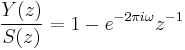
will give an overall transform of

The time-domain equivalent of this overall transform is
 ,
,
which becomes, assuming  for all
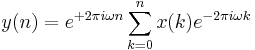
or, the equation for the  -sample DFT of
  , evaluated for and multiplied by the scale factor
  .
.
Note that applying the additional transform Y(z)/S(z) only requires the last two samples of the  sequence. Consequently, upon processing
  samples
  , the last two samples from the sequence can be used to compute the value of a DFT bin, which corresponds to the chosen frequency as

For the special case often found when computing DFT bins, where  for some integer,
  , this simplifies to

In either case, the corresponding power can be computed using the same cosine term required to compute as

Implementation
When implemented in a general-purpose processor, values for  and
and  can be retained in variables and new values of can be shifted through as they are computed, assuming that only the final two values of the sequence are required. The code may then be as follows:
s_prev = 0
s_prev2 = 0
normalized_frequency = target_frequency / sample_rate;
coeff = 2*cos(2*PI*normalized_frequency);
for each sample, x[n],
  s = x[n] + coeff*s_prev - s_prev2;
  s_prev2 = s_prev;
  s_prev = s;
end
power = s_prev2*s_prev2 + s_prev*s_prev - coeff*s_prev*s_prev2;
Instead of storing the history of samples in an array it is also possible to process the incoming samples iteratively in real-time.
Computational complexity
To compute a single DFT bin for a complex sequence of length N, this algorithm requires 2N multiplications and 4N additions/subtractions within the loop, as well as 4 multiplications and 4 additions/subtractions to compute  , for a total of 2N+4 multiplications and 4N+4 additions/subtractions (for real sequences, the required operations are half that amount). In contrast, the Fast Fourier transform (FFT) requires 2log2N multiplications and 3log2N additions/subtractions per DFT bin, but must compute all N bins simultaneously (similar optimizations are available to halve the number of operations in an FFT when the input sequence is real).
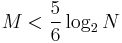
When the number of desired DFT bins, M, is small (e.g., when detecting DTMF tones), it is computationally advantageous to implement the Goertzel algorithm, rather than the FFT. Approximately, this occurs when
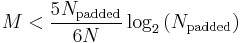
or if, for some reason, N is not an integral power of 2 while you stick to a simple FFT algorithm like the 2-radix Cooley-Tukey FFT algorithm, and zero-padding the samples out to an integral power of 2 would violate
Moreover, the Goertzel algorithm can be computed as samples come in, and the FFT algorithm may require a large table of N pre-computed sines and cosines to be efficient.
If multiplications are not considered as difficult as additions, or vice versa, the 5/6 ratio can shift between anything from 3/4 (additions dominate) to 1/1 (multiplications dominate).
References
- ^ Goertzel, G. (January 1958), "An Algorithm for the Evaluation of Finite Trigonomentric Series", American Mathematical Monthly 65 (1): 34–35
- ^ Mock (1985)
- ^ Chen (1996)
- ^ Schmer (2000)
- ^ http://www.dattalo.com/technical/theory/sinewave.html
- ^ http://cs-www.cs.yale.edu/c2/images/uploads/AudioProc-TR.pdf
- Chen, Chiouguey J. (June 1996), Modified Goertzel Algorithm in DTMF Detection Using the TMS320C80 DSP, Application Report, SPRA066, Texas Instruments, http://focus.ti.com/lit/an/spra066/spra066.pdf
- Mock, P. (March 21, 1985), "Add DTMF Generation and Decoding to DSP-μP Designs", EDN, ISSN 0012-7515, http://focus.ti.com/lit/an/spra168/spra168.pdf; also found in DSP Applications with the TMS320 Family, Vol. 1, Texas Instruments, 1989.
- Schmer, Gunter (May 2000), DTMF Tone Generation and Detection: An Implementation Using the TMS320C54x, Application Report, SPRA096a, Texas Instruments, http://focus.ti.com/lit/an/spra096a/spra096a.pdf
External links
- http://netwerkt.wordpress.com/2011/08/25/goertzel-filter/ C Code implementation of iterative Goertzel algorithm
- http://www.eetimes.com/design/signal-processing-dsp/4024443/The-Goertzel-Algorithm
- http://cnx.org/content/m12024/latest/
- http://www.embedded.com/showArticle.jhtml?articleID=17301593
- Proakis, J. G.; Manolakis, D. G. (1996), Digital Signal Processing: Principles, Algorithms, and Applications, Upper Saddle River, NJ: Prentice Hall, pp. 480–481